What To Do With All That Data

Session 9: What To Do With All That Data

You’ve got data. Lots of data. But it’s often messy, obscure, redundant or simply locked inside obnoxious proprietary file formats. Getting it clean and into the right shape so you can use it for your reporting is often the most excruciating part of the process. In this session, you will learn some basic, yet very powerful tools and techniques for importing, cleaning, transforming and extracting data. You will explore how to import and merge data and tables with Google Sheets, how to clean, transform, and explore data with OpenRefine, and how to extract tables from PDFs with Tabula.

Downloads

In this tutorial we will be using Google Sheets, as well as OpenRefine and Tabula. Both of those softwares are free to download and work on Macs, PCs, and Linux operating systems.

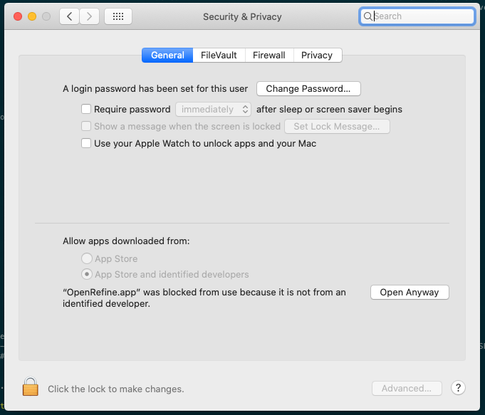
Once you download and install these softwares make sure you are able to open them: Mac computers might give you a notice that the software cannot be opened because the developer cannot be identified.

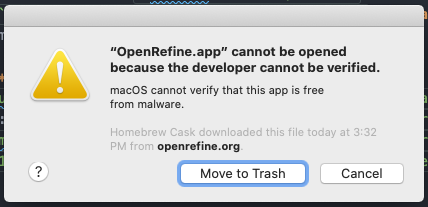
To open them, go to System Preferences / Security & Privacy / General and click Open anyway:

Data

To illustrate the different tools and techniques in this tutorial we will be working with data on three different topics: education, campaign finance, and police statistics. Please download the data package here.

This package includes the following datasets:

• Education data:
  • School Districts - Urban Institute Education Data Explorer: 2018 education districts (with enrollment) for New York State
  • SAIPE School District Estimates - US Census Bureau: 2018 population and poverty per school district for New York State
• Federal Election Commission data:
  • Individual Contributions by Individuals - Federal Election Commission: 2019 - 2020. The data package here includes a subset of this dataset, filtered to include only contributions to Kamala Harris campaign during a specific time period.
• New York City police statistics:
  • NYPD 2019 End of Year Enforcement Report

Importing Data and Joining Tables in Google Sheets

Google Sheets is an incredibly powerful and popular tool for working with small datasets. However, when using it you should be aware that you are uploading your data to Google’s servers. If you are working with data that must remain on your computer (for security reasons or other) you should not be using this tool. In addition, as with Excel, there is really no way to keep a systematic record of the different operations you will perform on your data on Google Sheets. If you need to reproduce your work or share your process with other people you won’t be able to do this while working with Google Sheets.

In this section we will work with the education data, which contains two different datasets, one with total number of students enrolled per school district and the other with total population, number of children, and children in poverty for each school district. We will join these two datasets and extract basic statistic from it.

First, open a new Google Sheets document and select File / Import. Choose Upload and select the SchoolDistricts_2018.csv file. In the import menu choose Replace spreadsheet as the import location, Comma as the separator type, and No for converting text to numbers, dates and formulas.

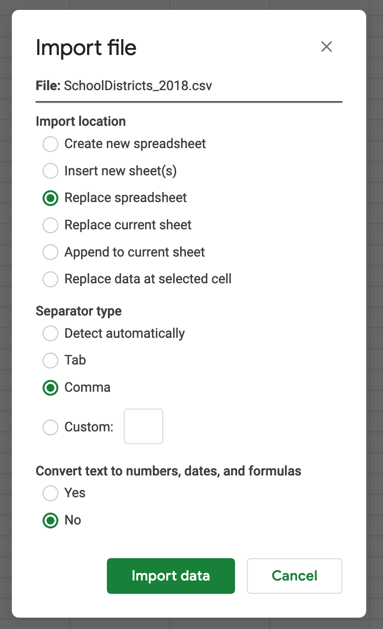
This last setting will ensure that whenever you have a piece of text that resembles a number, such as zip codes, it won’t be converted to numbers and loose any leading zeros. It is preferable to change text back to numbers than to try to change numbers or dates back to text.

Once we’ve imported the first dataset we can do some basic calculations:

• For example, we can get the total number of students enrolled by typing =SUM(G2:G1069) in an empty cell.
• Other common operations include getting the mean =AVERAGE(G2:G1069), median =MEDIAN(G2:G1069), and standard deviation =STDEV(G2:G1069).

You can also create filters on your dataset and filter and sort by each column. To do this click on the funnel button on the top menu. Once there you can click on each header cell to sort ascending or descending or filter out certain values.

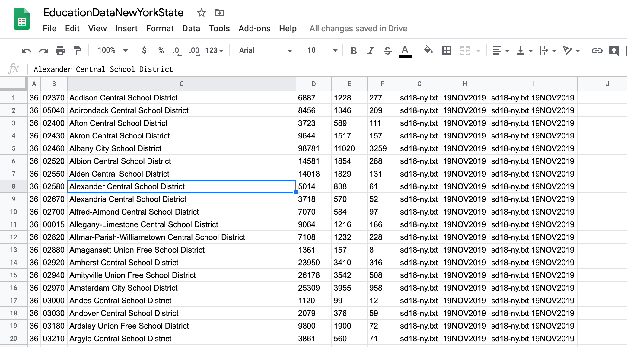
Next, import the other education dataset (SAIPE School District Estimates). For this one, though, choose Insert new sheet as the import location so that it is imported into the Google Sheet we are working with, and Detect automatically as the separator type.

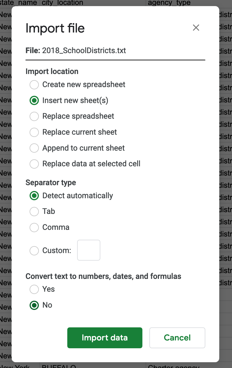
This file is actually a Fixed width file where instead of using a specific character to separate columns (commas, tabs, etc), each column has a fixed with. Google Sheets is smart enough to detect this kind of separation (almost perfectly).

If you look at the 2018_SchoolDistricts_Layout.txt file you will notice that the last column contains both the file name and the date on which it was created. Google Sheets actually divided this column into two separate ones. To join the two columns (following the original file) type =G1&" "&H1 in the I1 cell. Then copy and paste this formula all the way down.

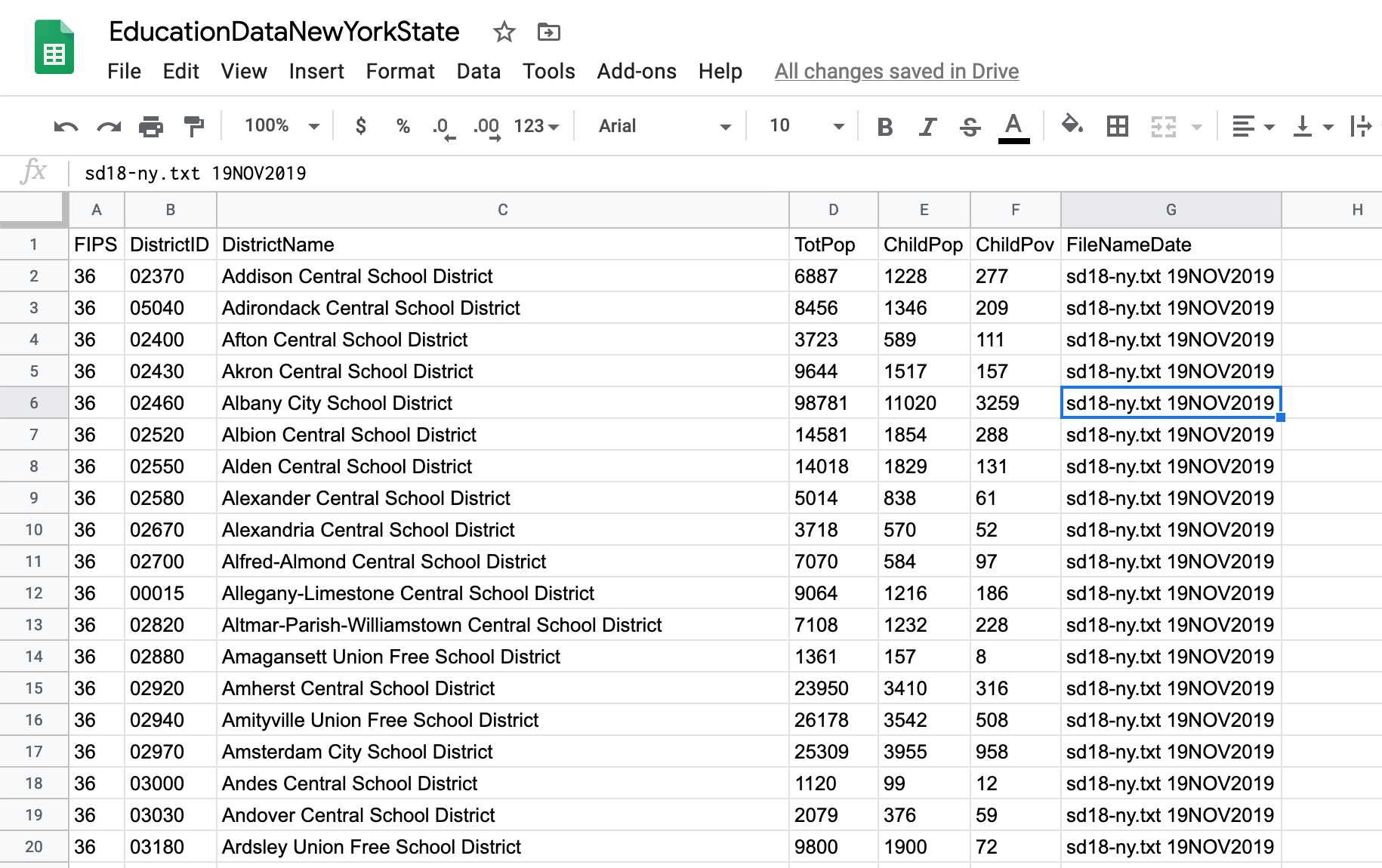
Next, so we keep these values independent of the formula or other columns, copy and right-click and choose Paste special / Paste values only on the column, and delete the other two.

Now insert a row at the top and add the headers from the original file.

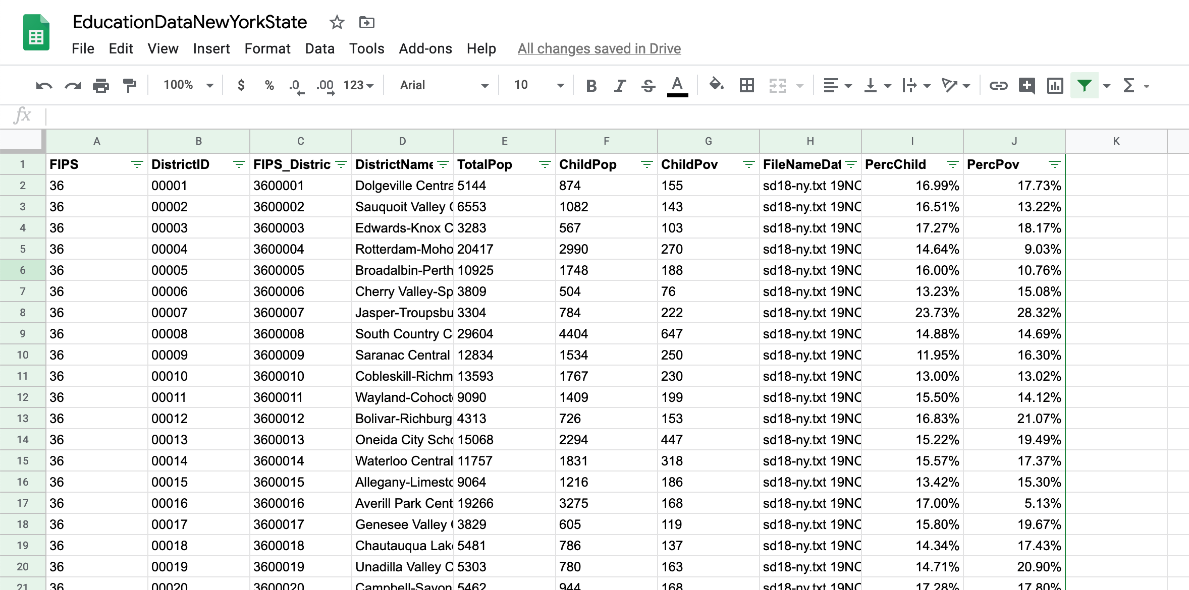
Next we can calculate the percentage of children in each school district, as well as the percentage of children in poverty:

• =F2/E2 and =G2/F2

Now let’s join the two files. We will do this using the leaid column from the school district file and a combination of the FIPS and DistrictID columns in the school districts estimates file.

First, we need to combine the FIPS and DistrictID columns. Do this by inserting a new column and adding the following formula: =A2&B2. As above, copy the formula down and then replace the column by copying and pasting only the values.

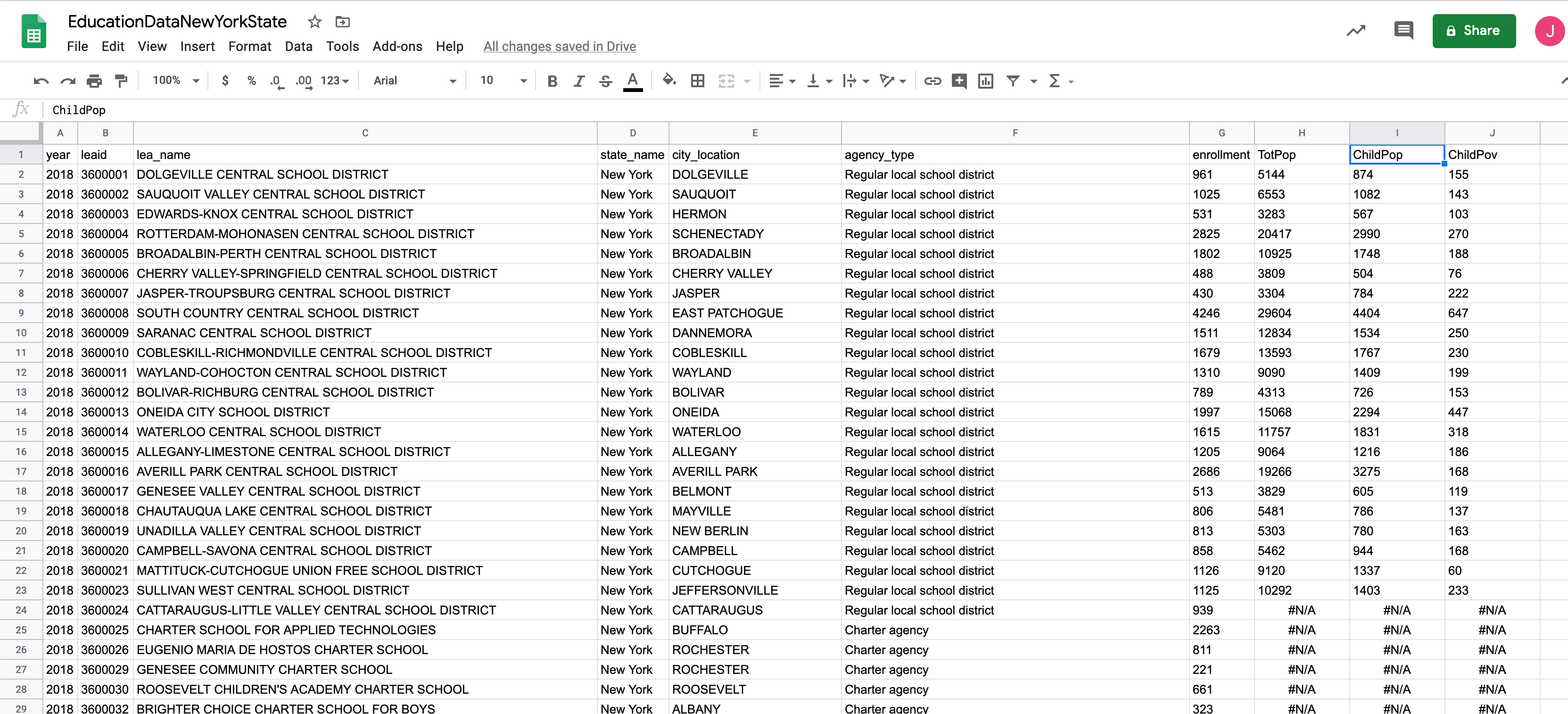
Now let’s do the actual join: let’s bring in the total population data. In the school districts tab, on a new column, type the following formula: =VLOOKUP(B2,'2018_SchoolDistricts'!$C$2:$J$683,3,false). Here we are using the VLOOKUP function, which looks up a value on a specified range and then returns another value from the row that matched the lookup value.

Here’s how the formula’s arguments work: =VLOOKUP(valueToLookup, lookupRange, columnPositionOfValueToReturn, useApproximateMatch).

• The last argument (false in our case) makes sure the formula only returns a value when there’s an exact match, which is probably what you will want in most cases.
• The various $ (dollar signs) in the lookup range make sure the range won’t change as you copy the formula to other cells.

Once you do this you will see many values populating but many others returning #N/A. That is because school districts with charter agencies don’t cover a specific geographic area and thus don’t have a specific population.

Do the same operation for the other two data columns: children and children in poverty.

Once you’ve brought the data through the VLOOKUP function, replace the formulas by copying and pasting only the values.

Now let’s get some small insights out of this data by using IF statements.

For example, let’s figure out how many entries with Charter agency as the agency type there are. In an empty cell type =IF(F2="Charter agency",1,0). Now copy the formula down and add up all the 1s.

The IF statement is a very simple formula, but you can use it as the basis for more complex queries. In this case, we can also use a variation of this formula: in another cell type =COUNTIF(F2:F1069,"Charter agency"). This formula specifically counts if the selected cells match the provided criteria.

But the criteria don’t always need to be text, they can also be numerical. For example, count the rows where the enrollment is greater than 999 with =COUNTIF(G2:G1069,">999").

Or sum the enrollment in Charter agency rows with the SUMIF variation of the IF formula: =SUMIF(F2:F1069,"Charter agency",G2:G1069). You might not get a result because Google Sheets is still treating the numbers in the enrollment column as text. To change that select the whole column and go to Format / Number and select Number. Now the formula should work.

Go ahead and convert all numerical columns to Number in the same way.

You can also use multiple conditions to get a result, for example, sum all the enrollment in rows with Charter agency and BRONX as city_location. Here you should use the SUMIFS function, which takes as many ranges and conditions as you want to give it: =SUMIFS(G2:G1069,E2:E1069,"BRONX",F2:F1069,"Charter agency").

And if you want to sum all the enrollment in Charter agencies for New York City (except for Queens, which is not specified as such) you can use multiple SUMIFS functions. This will be the same as saying something like: sum if the agency type is charter and city location is Broonx, or Brooklyn, or New York, or Staten Island. This is how you write this formula:

=SUMIFS(G2:G1069,E2:E1069,"BRONX",F2:F1069,"Charter agency") + SUMIFS(G2:G1069,E2:E1069,"BROOKLYN",F2:F1069,"Charter agency") + SUMIFS(G2:G1069,E2:E1069,"NEW YORK",F2:F1069,"Charter agency") + SUMIFS(G2:G1069,E2:E1069,"STATEN ISLAND",F2:F1069,"Charter agency")

Finally, let’s look at Pivot Tables. These are extremely powerful types of tables that aggregate and filter your data and that you can configure in a variety of ways to extract insights.

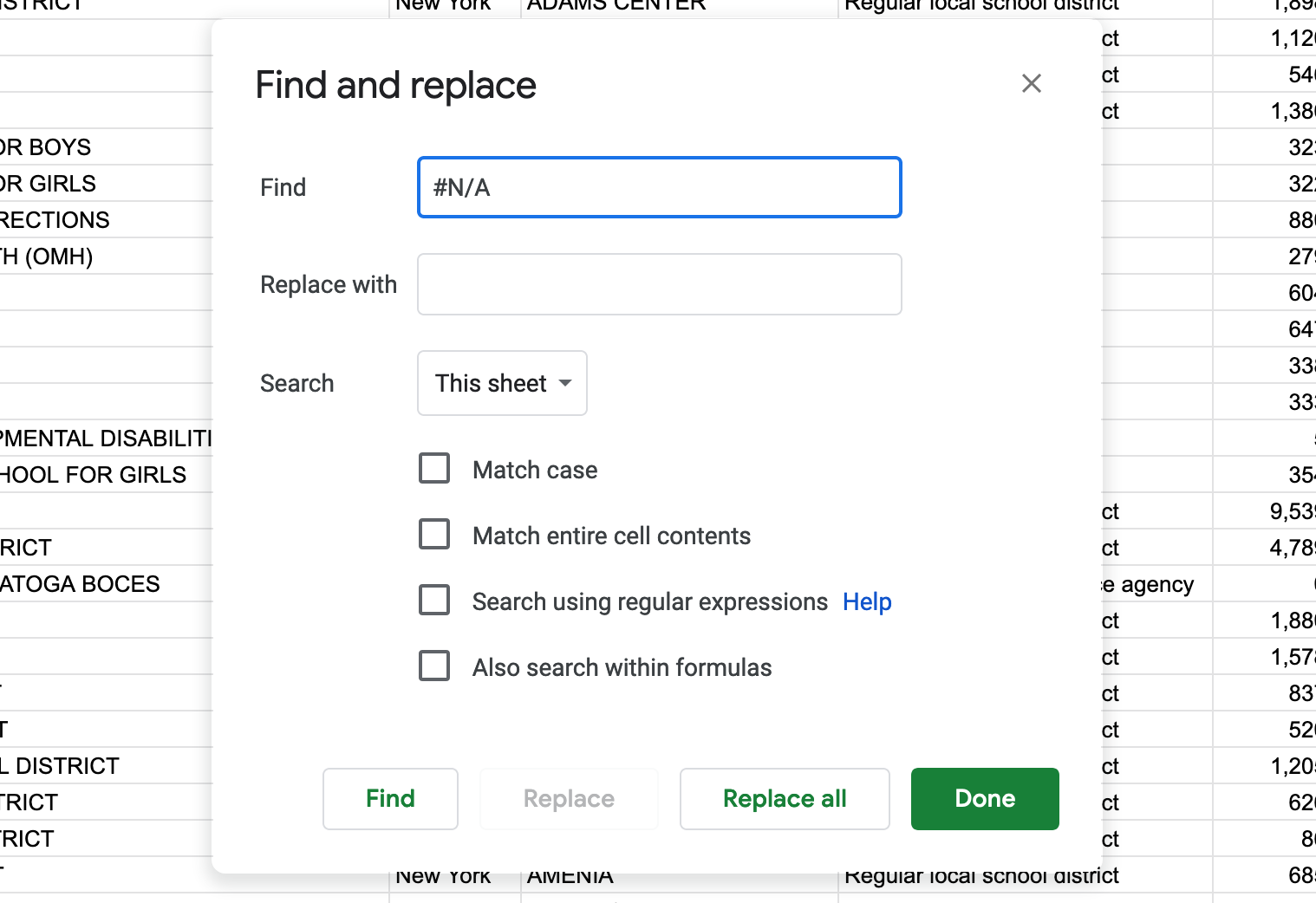
Before we create a Pivot table we need to replace all the #N/A values with nothing. Do this by clicking on Edit / Find and replace and typing #N/A in the find field. Leave the replace with field empty. In the search dropdown menu choose This sheet. Finally, click on Replace all and then Done.

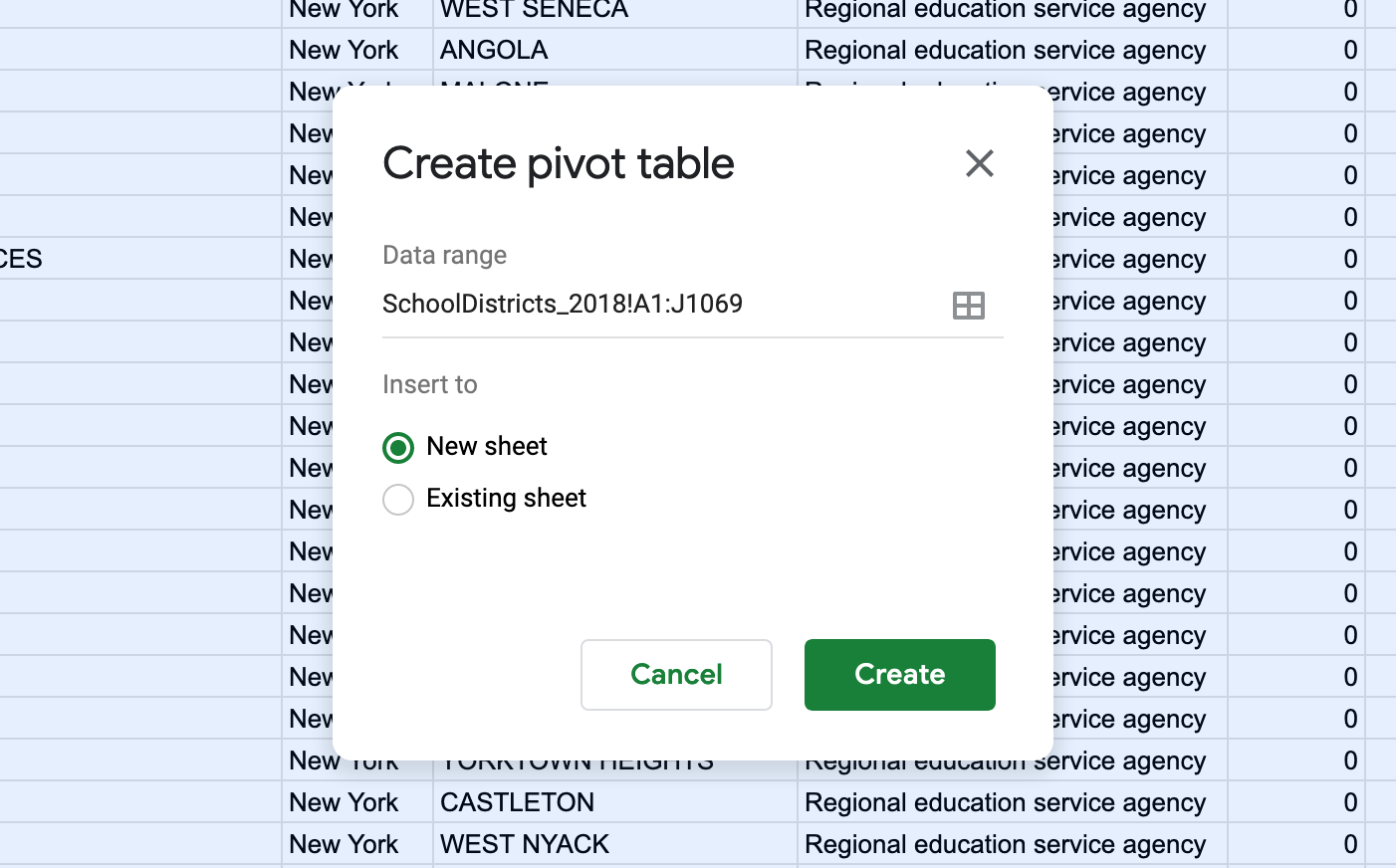
Now to create a Pivot Table select all the data in your Google sheet and click on Data / Pivot table. Make sure that the data range is correct and add your pivot table into a new sheet.

In the new sheet you will have a menu on your right-hand side that controls the pivot table. There you can select fields as columns, rows, filters and values. In addition, here you will be able to specify how your data will be aggregated (sum, count, percentage), how it will be ordered, and how it will be displayed in the table.

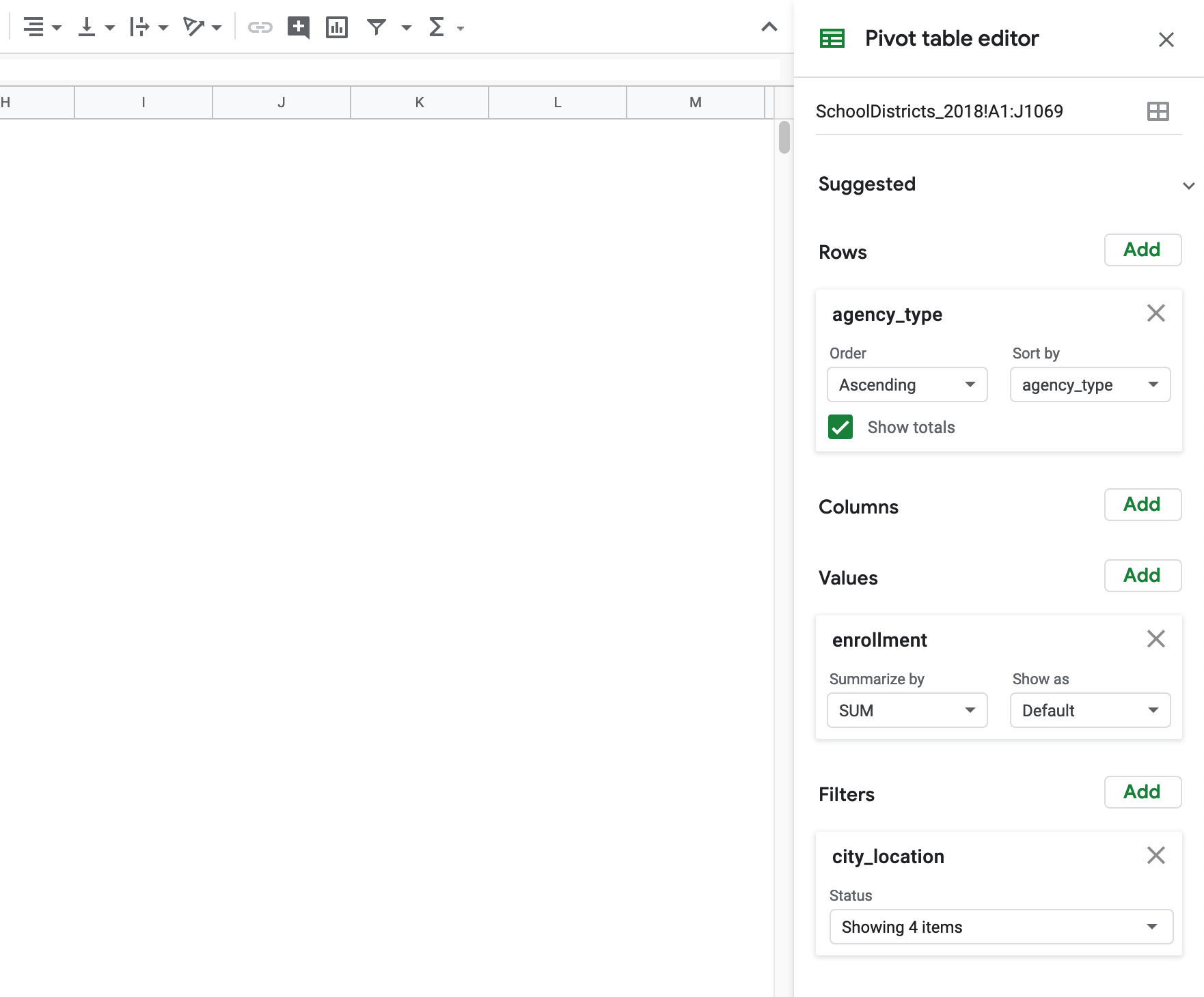
Go ahead and experiment with the pivot table and recreate all the analysis we did before with the IF statements. Once you get an insight you would like to keep, I suggest copying the table and pasting values only in another sheet. That way the values will stay fixed even if you reconfigure your pivot table. Usually, we do this multiple times extracting as many valuable insights as we can.

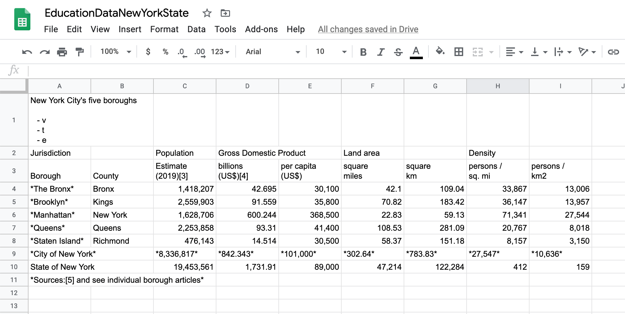
Finally, one last very useful tool included in Google Sheets is the ability to import tables and lists from other websites directly into your sheet. For example, it would be great if we could import data from this Wikipedia page with the population for every New York City borough.

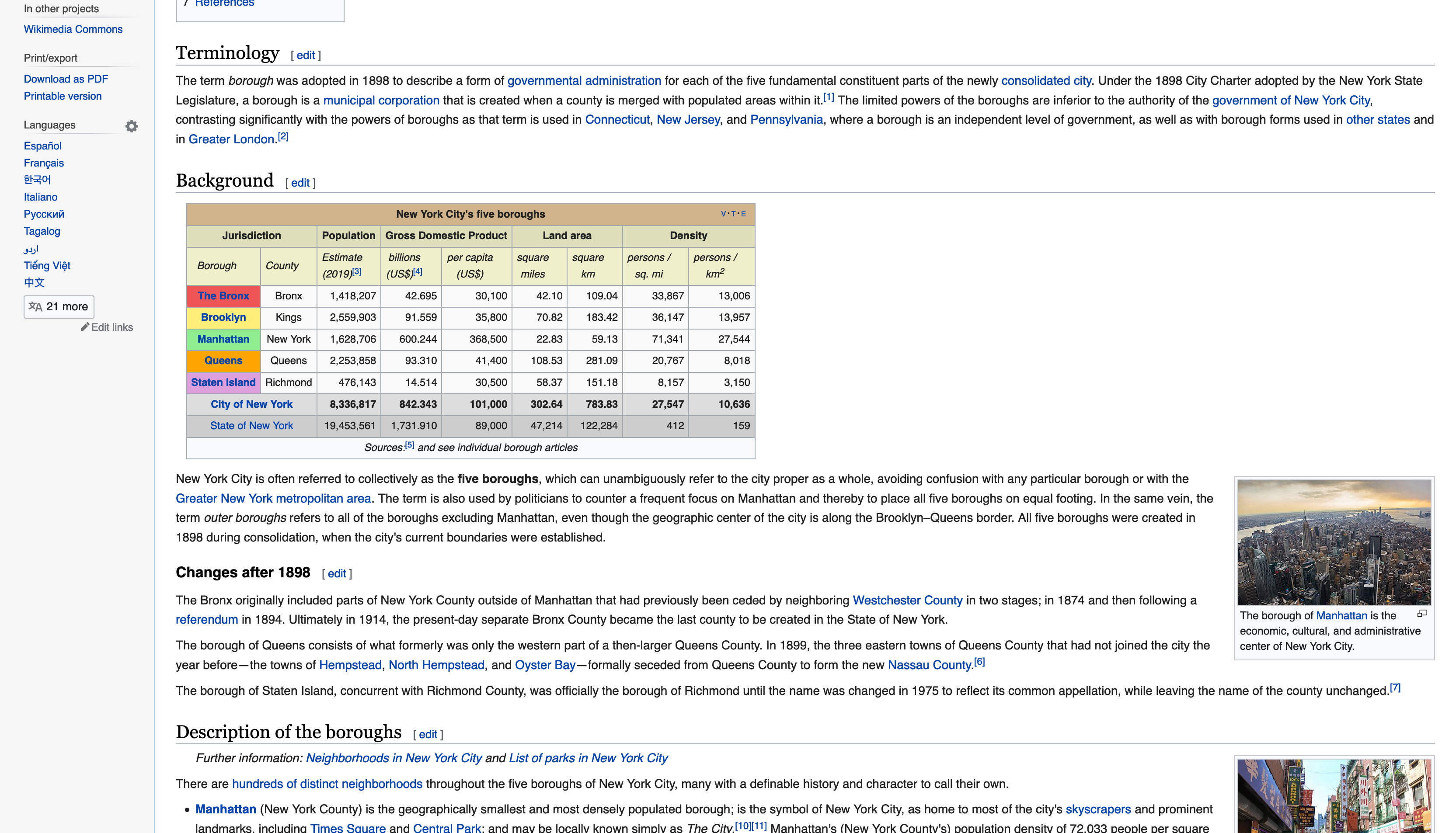
To do this, create a new sheet and on its first empty cell type the following formula: =IMPORTHTML("https://en.wikipedia.org/wiki/Boroughs_of_New_York_City","table",1). This will look at the page and identify the first table. If we wanted to import the second table you would just change the last argument of the formula to 2. If you wanted to import the first list, you would change the second argument to list. Just make sure that the first and second arguments (URL and table or list) are both inside double quotes. And usually it takes a few tries until you get the right table or list you want to import.

The result is a table in your sheet. Maybe not the best formatted table, but much much better than manually copying the values.

Finally, exporting your Google Sheet is pretty simple. Just click on File / Download and choose your desired format. The most common format for data files is csv (comma separated values), as well as tsv (tab separated values). Note that these two formats only export the current sheet. If you export as an Excel file you will get your whole Google Sheet document with all the tabs.

Importing, Cleaning and Joining Data with OpenRefine

OpenRefine (formerly Google Refine) is an amazing tool to work with on the first stages of any data analysis project. However, it is specially powerful when working with messy textual data. In this part of the tutorial we will reproduce most of what we just did in Google Sheets in OpenRefine and then we will use the campaign finance data to test some of OpenRefine’s more powerful data cleaning tools.

First, open OpenRefine (if you get a warning saying that the software cannot be opened please see the explanation at the top of this tutorial). The first thing you will notice is that OpenRefine actually opens in your browser, using an 127.0.0.1 URL. This means that even though you are using OpenRefine through your browser, the program is running locally. OpenRefine actually creates a local server on your computer and opens your browser pointing to that server. Ultimately, this means that everything you do or ‘upload’ to OpenRefine stays on your computer. This is specially convenient when dealing with sensitive data that can’t be uploaded to the cloud.

To import a file, first create a project. Select the school districts file. Once you’ve selected the file to ‘upload’ you will see the import menu. here you will be able to specify the type of delimiter (commas), if the first row contains the headers (yes), and many other import options. You can see that OpenRefine can import a variety of data types, from the most common csv or tsv files, to the more obscure fixed-width or even RDF files.

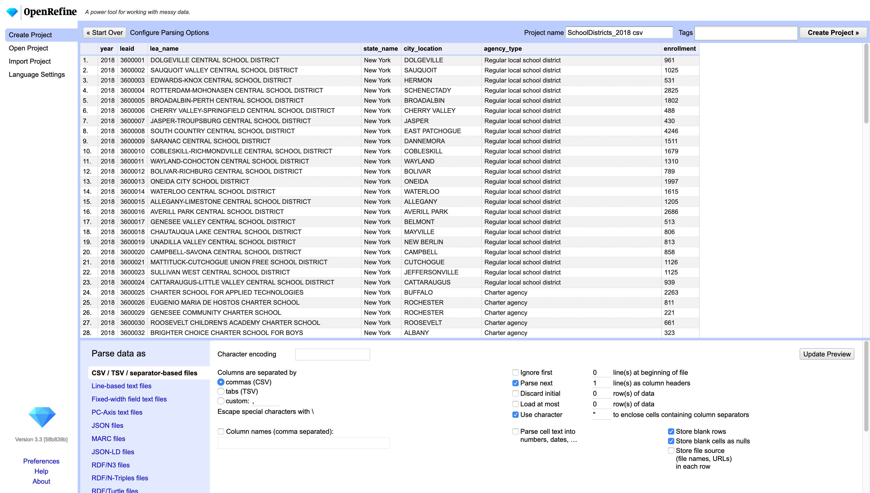
Once you’ve selected the right import settings, click on Create project. Note that OpenRefine will only show you 10, 20 or 50 rows, depending on your settings. This doesn’t mean your dataset got cut. All the rows are there.

Next, create another project and import the school districts estimates file. This one will be a fixed-width delimited file and you will see how OpenRefine allows you to manually move the divisions between columns. You can also type in the exact width of each column in at the bottom of the import menu. For this file, the column widths are 2,6,73,9,9,9. That is the number of characters in each column.

Once you’ve imported this second file, let’s rename the columns. To do this, click on the dropdown menu at the top of each column and choose Edit column / Rename this column.

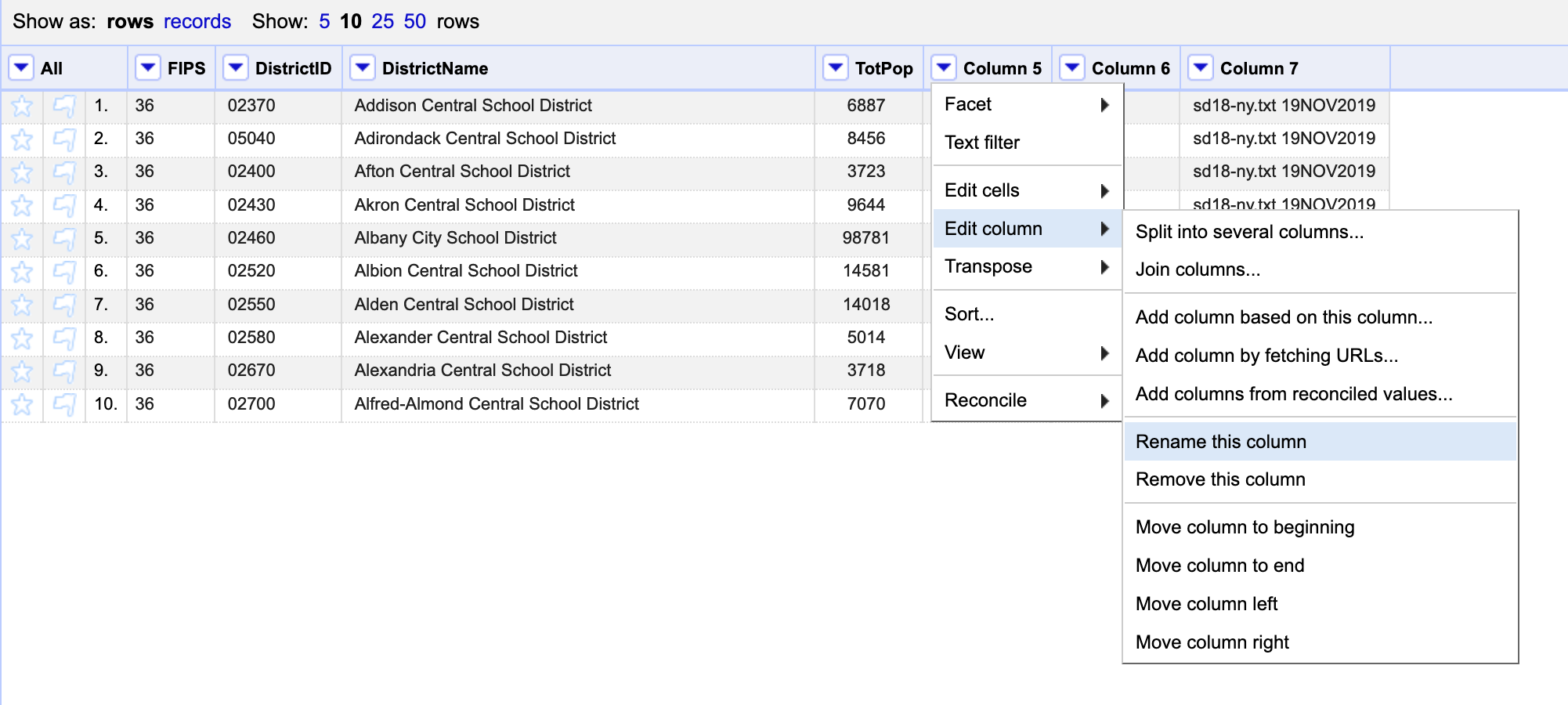
After renaming the columns, let’s create the FIPS_DistrictID column that will allows to join this dataset with the school district one. To do this click on either the FIPS or the DistrictID column and select Edit column / Join columns. Here you will be able to select the columns to join, rearrange their order, add a separating character (if necessary) and name the new column, amongst other things. Select the two columns we want and name the new column FIPS_DistrictID.

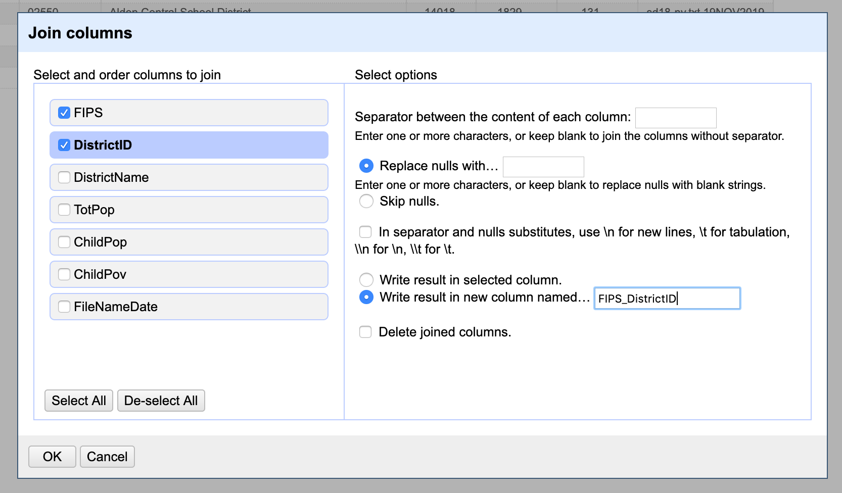
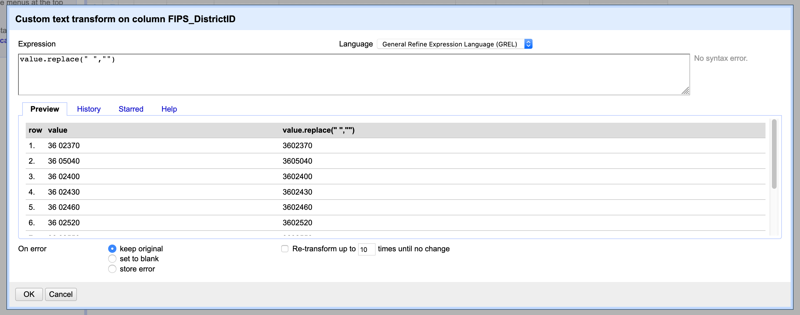
Now you’ll notice that the new column includes a space between the FIPS code and the DistrictID code. To get rid of this space we will write a tiny bit of code. Click on the new column dropdown menu and choose Edit cells / Transform. Here you will get a menu where you can type in an expression to transform the cells in this column. In the expression box type value.replace(" ","") which will replace any " " value with nothing.

In this same window you will be able to see a sample of what this transformation will look like and set how this formula will deal with any errors.

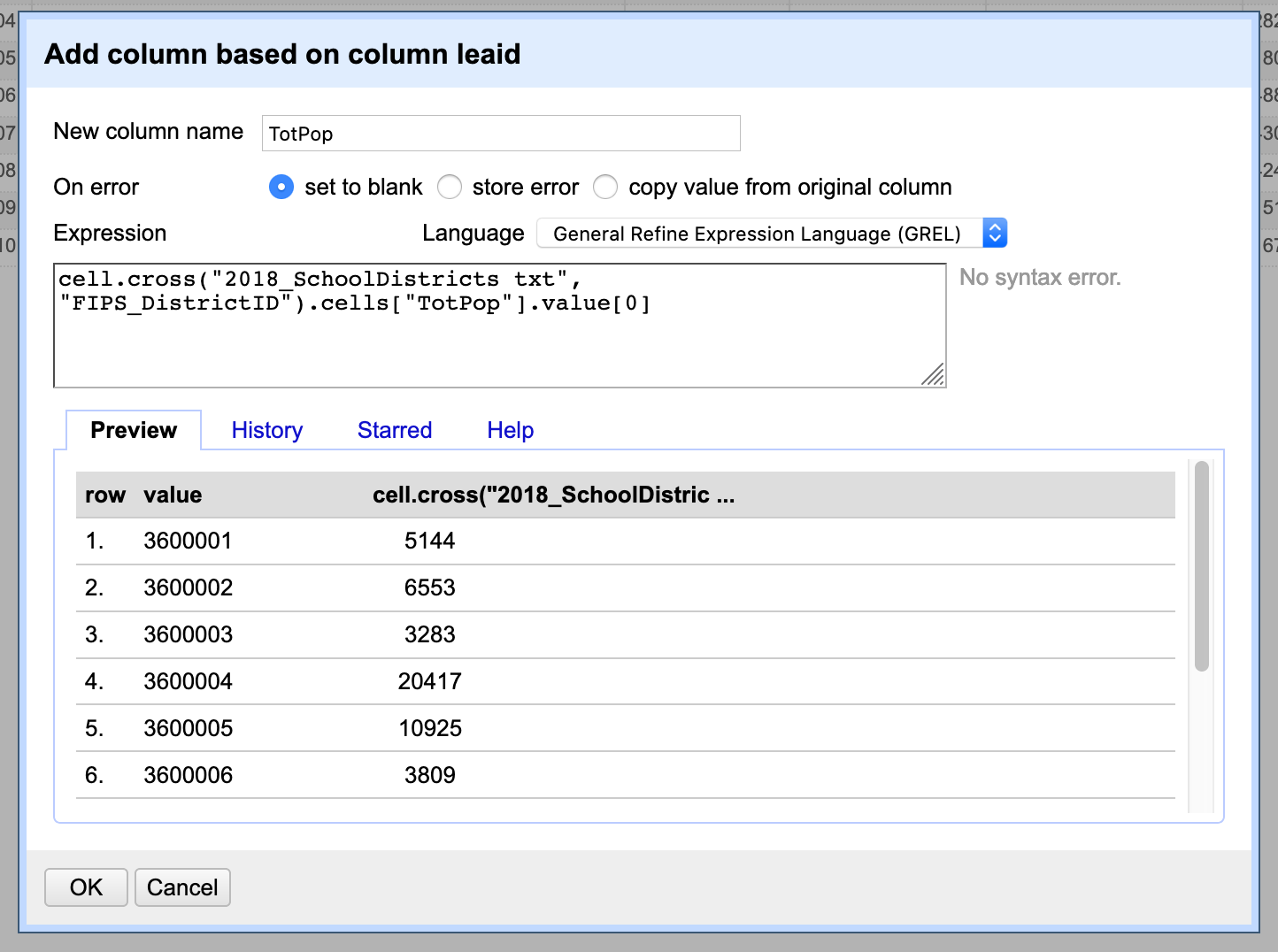
Next, we need to create a new column on the school district dataset that will bring in the population field from the estimates dataset. To do this click on the FIPS column dropdown menu and select Edit column / Add column based on this column. On this window add the name of the new column (TotPop) and in the expression box type the following formula: cell.cross("2018_SchoolDistricts txt", "FIPS_DistrictID").cells["TotPop"].value[0]. This formula cross references the values in this column with the values in the FIPS_DistrictID column in the 2018_SchoolDistricts txt project, and brings in the TotPop values.

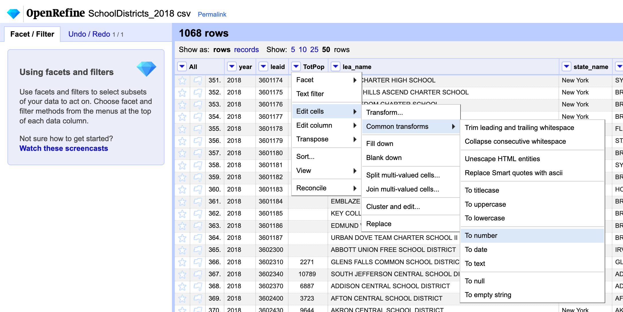
Once we bring in the population data we should convert it to a number. To do this click on the column dropdown menu and choose Edit cells / Common transforms / To number. Here you can see a list of other common types of transformations. Many of these are extremely useful, specially when working with messy textual data. Do this for the population column as well as for the enrollment one.

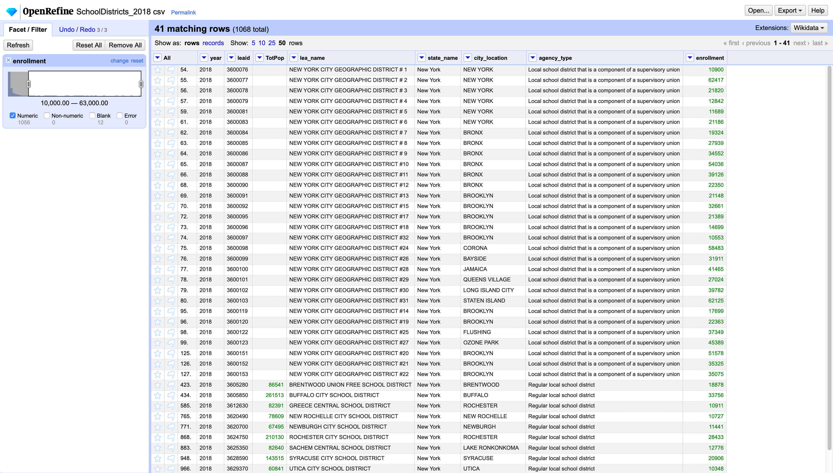
Now that the enrollment column is of number type we can create a Number facet and see a histogram of the values in this column. Click on the dropdown menu for the enrollment column and select Facet / Numeric facet. This will create a histogram of the data on the left hand panel that you can use to filter the data by their value. Here you see that there are 12 rows with blank values as well as 1056 with numeric values. You can also see that the values go from 0 to 63,000 and that most of the values are concentrated in the lower bounds.

If you wanted just to export the school districts with more than 10,000 students you could use the sliders in this facet to filter only those value and then export the dataset.

The same way we can filter or facet by number, we can facet, filter, and transform using textual fields. Let’s use the facets to convert the locations in Queens to “QUEENS” instead of “BAYSIDE”, “ASTORIA”, etc. First, create a textual facet on the agency_type column. In the facet, select only Local school district that is a component of a supervisory union. This will filter down your dataset to 33 rows. Next create another facet on the city_location column. Here choose BAYSIDE, CORONA, FLUSHING, JAMAICA, LONG ISLAND CITY, OZONE PARK, and QUEENS VILLAGE.

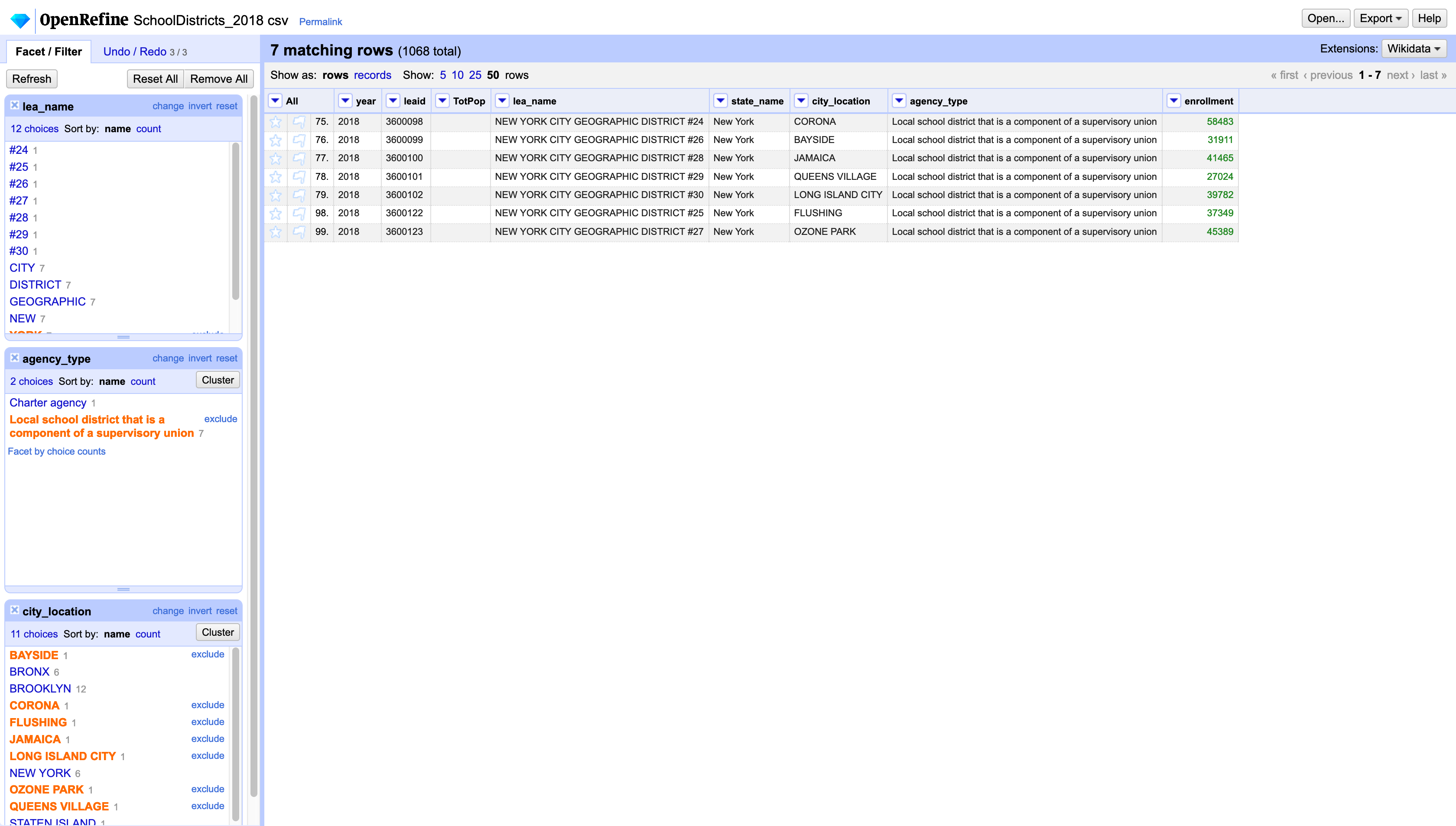
Once you have only those records selected, click on the city_location dropdown menu and choose Edit cells / Transform. In the expression field, just type "QUEENS". This will transform all those values to the borough name.

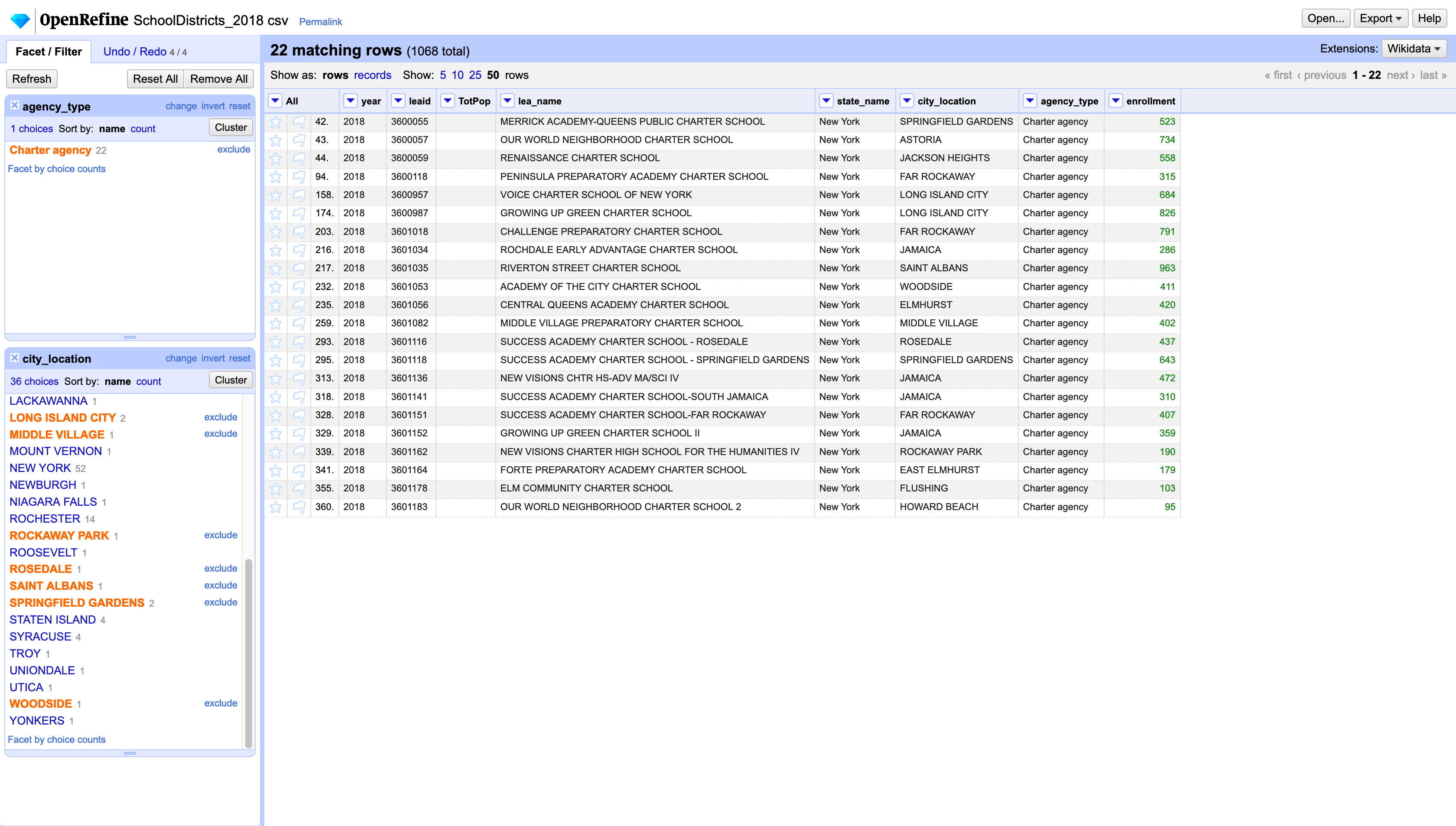
Next, clear the facet for the city_location column and change the facet for the agency_type to include only Charter agency. The city_location facet will now include many more options. Select the following and change them to QUEENS: SPRINGFIELD GARDENS, ASTORIA, JACKSON HEIGHTS, FAR ROCKAWAY, LONG ISLAND CITY, JAMAICA, SAINT ALBANS, WOODSIDE, ELMHURST, MIDDLE VILLAGE, ROSEDALE, EAST ELMHURST, and HOWARD BEACH.

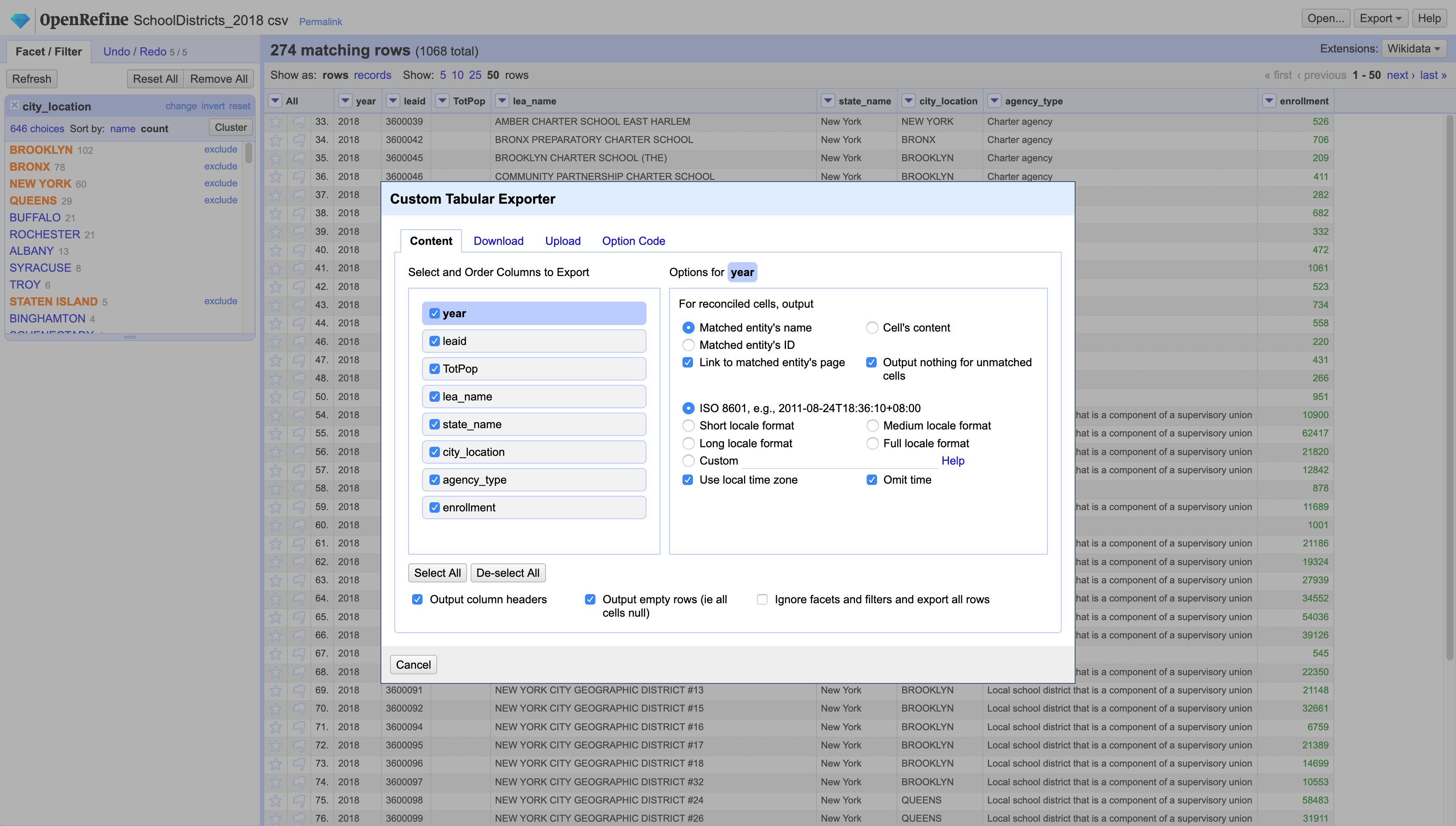
Finally, once you’ve changed all those values to QUEENS, use the city_location facet to select only the records that correspond to the 5 boroughs in New York City. Now you can export only these rows to get all the data for New York City. Click on the Export button at the top-left corner. You can click on the preset options or if you want to customize your export you should select Custom tabular exporter. Here you will be able to choose what columns you want to export, and for each of those columns a few more options, what format you want to export to, what delimiter you want to use, and other settings.

Now let’s change datasets to explore the more advanced text tools in OpenRefine.

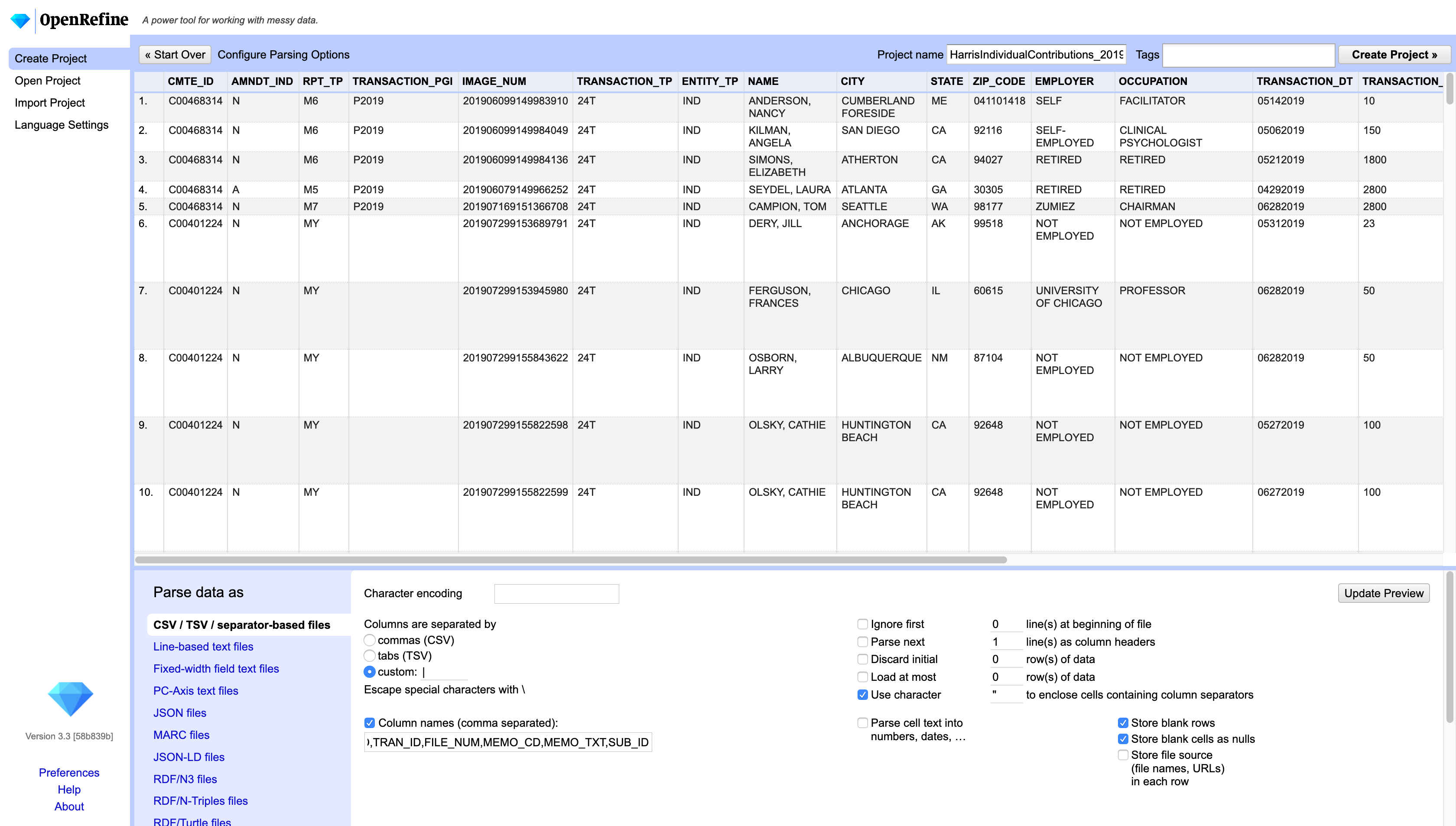
Create a new project and import the campaign finance dataset. Make sure to add the column names in the import menu. The names for these columns can be found in the data dictionary for this file.

This file contains the names of individual contributors. To correct misspelling of these names we will use the text facet and the cluster option. Create a textual facet on the NAME column and then choose Cluster (this operation might take a bit of time). Once the initial search is done you will get a window showing all the possible clusters found in the data. There are many methods to create the clusters. You should experiment with them and choose the one that best works for the kind of data you are working with. For a more detailed explanation of the cluster algorithms see OpenRefine’s documentation.

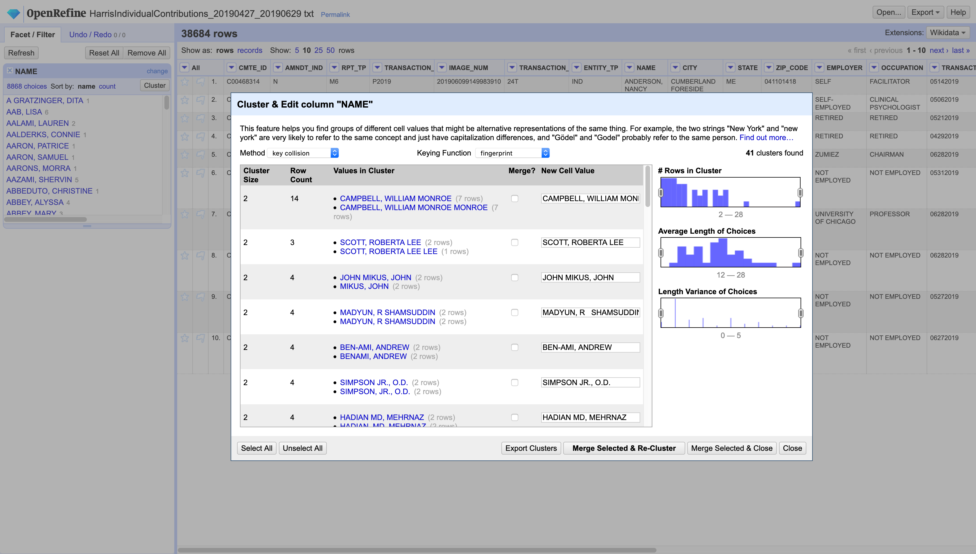
Double check that all the clusters make sense, select the ones that you want to change, make sure the replacement value is correct and hit Merge Selected & Re-Cluster. This will merge the selected clusters and search again in case this yields new clusters. Do this until you are satisfied and then hit Close.

Do the same for the EMPLOYER and OCCUPATION columns.

Next, tRansform the TRANSACTION_DT column to date and the TRANSACTION_AMT to number. Now you can create facets on those columns and explore how the data is distributed by date and by amount. You will even find some negative values in the transaction amounts.

Finally, export a clean version of this dataset.

Note that on the left hand panel, under Undo / Redo you can see all the operations you’ve performed on your data. This is one of the great features of OpenRefine. Here you can undo, or redo operations, as well as export these and share them or apply them to other datasets. Also, and very important for data journalism, you are able to document and reproduce your steps.

To see all stored projects on your computer click on Create project / Open project and click on the Browse workspace directory with the link at the bottom of the page.