Intermediate Python
Session 5: Intermediate Python
Here’s a video recording of the session:
Review - Web Scraping
We begin where Alex left off last week — with web scraping. For those of you who couldn’t attend his session, “web scraping” involves taking data that was formatted for one purpose and translating it for another. Let’s take a simple example. My Computational Journalism Class has been helping the Detroit Free Press automate some of the statistics it collects from the Michigan Government about COVID-19.
Tracking
For example, coarse county-level statistics about the number of cases are available through the state portal. Click through on the button labeled “SEE CUMULATIVE DATA” and you’ll find a page of tables. As it turns out, grabbing these data is easy. Have a look at the underlying HTML source code and you’ll find that the page is filled with proper <table>’s. Here is the first table, the breakdown of incidents by county.
<table border="1" cellpadding="0" cellspacing="0" style="width:100%;" width="561">
	<thead>
		<tr>
			<th height="22" scope="col" style="height: 22px; width: 197px; text-align: center;">County</th>
			<th scope="col" style="width: 189px; text-align: center;">Confirmed Cases</th>
			<th scope="col" style="width: 175px; text-align: center;">Reported Deaths</th>
		</tr>
	</thead>
	<tbody>
		<tr height="22">
			<td height="22" style="height: 22px; width: 197px; text-align: center;">Alcona</td>
			<td style="width: 189px; text-align: center;">4</td>
			<td style="width: 175px; text-align: center;">1</td>
		</tr>
		<tr height="20">
			<td height="20" style="height: 20px; text-align: center;">Allegan</td>
			<td style="text-align: center;">116</td>
			<td style="text-align: center;">2</td>
        </tr>
    ...
		<tr height="22">
			<td height="22" style="height: 22px; text-align: center;">Totals</td>
			<td style="text-align: center;">43950</td>
			<td style="text-align: center;">4135</td>
		</tr>
	</tbody>
</table>
These we can pull simply using Google Sheets! Remember the function IMPORTHTML(). Focusing on this same first table of county breakdowns we can do the following.

Every table on this page is formtted using <table> tags and can be brought directly into Google Sheets. Here we look at the sixth table which presents the racial breakdown of COVID cases.

As Alex discussed last week, data on web pages aren’t always nicely arrnged in <table>’s. On the Michigan main coronavirus page, for example, they have this interactive display with total case numbers for the state on the right.

The underlying HTML for this part of the page looks like this.
<section class="stat-container">
<p class="stat-title-text" style="text-align: right;">Total Confirmed Cases</p>
<p class="stats-text" style="text-align: right;">43,950*</p>
<p class="stat-title-text" style="text-align: right;">Total COVID-19 Deaths</p>
<p class="stats-text" style="text-align: right;">4,135*</p>
<p class="stat-title-text" style="text-align: right;">Daily Confirmed Cases</p>
<p class="stats-text" style="text-align: right;">196*</p>
<p class="stat-title-text" style="text-align: right;">Daily COVID-19 Deaths</p>
<p class="stats-text" style="text-align: right;">86*</p>
<p class="stats-text" style="text-align: right;"> </p>
<p style="text-align: right;">Updated 5/4/2020</p>
...
</section>
The class information is what makes the data look different on the page. As Alex discussed, this is done using CSS or Cascading Style Sheets. Here are the styling entries for the statewide statistics. They are included with the page itself, although in many cases the styling is kept in a separate file so that it can be used to style statistics, say, across the site for an overall “look and feel.” Here’s the styling or CSS specification.
.stats-text {
    font-family: montserrat, sans-serif;
    font-size: 3.5rem;
    font-weight: 700;
    line-height: 4rem;
    margin: 0;
    padding: 0;
    color:#0077A7;
 }
 .stat-title-text {
    font-family: montserrat, sans-serif;
    font-size: 1.5rem;
    line-height: 1.7rem;
    margin: 0;
    padding: 0;
 }
We see that any tag with a class stat-title-text (denoted by the “.” in front of the classname) is rendered 1.5 times the size of the “root element”. Put another way, it’s 1.5 times bigger than the base font, making it stand out from the page. By contrast, the stat-text is 3.5 times the size of the root element, making it really big. The color for the statistics has also been specified in the styling. It’s a blue-green #0077A7.
And here’s the trouble with using HTML to transmit data. The markup language was designed to help you make documents, not store or transmit data for other people to use. The designer of the page decided to use separate paragraphs to present statewide statistics, and then applied simple styling rules to say how the text in these paragraphs should be formatted. But as a data journalist, your interest is less in the styling as a way of making the data look nice, but instead that it provides a direct pointer to the text and numbers we want on the page. To pull these data from the web page, then, we need to parse the HTML and look for <p> paragraphs that alternately have class stat-title-text and stats-text.
Alex showed you how to write a program to do this using a Python package called BeautifulSoup.
from requests import get
from bs4 import BeautifulSoup

# Michigan's main coronavirus page
url = "https://www.michigan.gov/coronavirus"

# pull the HTML page...
response = get(url)

# ... parse it using BeautifulSoup
soup = BeautifulSoup(response.text)

# find all the <p> paragraph tags with class 'stats-text'
stats = soup.find_all("p","stats-text")

# and print them out (they're a list!)
stats
# or process them one at a time in a loop

for stat in stats:
    print(stat.text)
From here, we might have to clean things up a bit. We would want to remove the asterisks, for example, that are referring to notes about the day’s data at the bottom of the display. As an aside, we wouldn’t know to collect those notes because they are just another <p> paragraph tag and we could easily miss them. This is another downfall of using tags designed to format documents and not some other real data structure that would have a place for us to store important notes.
Still, once we have a piece of Python code that pulls these numbers and their descriptions, we can do it everyday and add them to a Google Sheet using the sheets package.

This code is running daily for the Detroit Free Press and something like it is running in newsrooms across the country, pulling down data from government agencies or other organizations, slowly, day by day, compiling the informtion into something that can be studied across time. The pipeline is easy to create — we spun up an EC2 machine from Amazon, put our code on the machine and set a cron job to pull the page every 15 minutes, checking for new statistics. If it finds them, it adds them to the top of the sheet.
By the way, not all the work you’ll do necessarily involves parsing HTML. Sometimes, when the data are trapped in an interactive display, they are communicated separately — a piece of JavaScript code running in the browser might make a request to a Michigan server, say, for data about Oakland County. Using the “JavaScript Console” on Chrome, say, you can see all the data your browser is requesting.

For Oakland County, the map’s data comes from a call to the URL below. It’s ugly, but it has the goods. The data it returns is in the form of a JSON string, where JSON stands for JavaScript object notation. If you remember our first session, JSON will look like a dictionary with the built-in data types like numbers and strings and lists and, yes, other dictionaries.
Let’s look at the Oakland data.
# The URL for the JSON map data
url = 'https://services1.arcgis.com/GE4Idg9FL97XBa3P/arcgis/rest/services/COVID19_Cases_by_Zip_Code_Total_Population/FeatureServer/0/query?f=json&where=1%3D1&returnGeometry=false&spatialRel=esriSpatialRelIntersects&outFields=*&orderByFields=Join_Zip_Code%20asc&resultOffset=0&resultRecordCount=200&cacheHint=true'

# get() the data from the server
response = get(url)

# this time, instead of using response.text, we use a built-in feature of the package
# and extract the parsed JSON already. think of it as returning a dictionary rather
# than a string as response.text would.
data = response.json()

# and have a look -- remember it seems a bit ugly at first
data
This is a dictionary with a lot of keys. (We know it’s a dictionary because the whole mess is enclosed in curly braces.) We see fields and geometryType, the sorts of things that indicate the data have something to do with maps. If you poke around a little, you’ll see that under the key features, you find the pieces of the map we want.
data.keys()
data["features"]
So under the key features we have a list. We know it’s a list because it is surrounded by square brackets. We access list items by number, starting with the first assigned the value 0.
data["features"][0]
data["features"][20]
As with the state summary statistics, we have a process running every 15 minutes, grabbing this file and looking for changes. The whole thing is updated on a Google Sheet using the Python package sheets that the Free Press then pulls from to populatetheir graphics.
Impacts
Last week, Alex showed you that sometimes things can be harder than this. He studied the WARN (Worker Adjustment and Retraining Notification Act) reporting site for New York State. Essentially WARN is a federal labor law that required employers with more than 100 employees give notice before plant closings and mass layoffs. Have a look at the NYS WARN site. It posts all the data coming from New York State on layoffs. Our interest today is what this says about COVID’s impact on the local economy. Here is the site.

You’ll see the individual WARN notices at the bottom of the page. If you inspect the source, you’ll see that they are in a large table. Great! Right?
<table width="95%" cellspacing="0" border="0" align="center"
            bgcolor="#FFFFFF" bordercolor="#000033" cellpadding="4">
	<tr>
		<td>
            <span class="style2">
                <font face="Arial, Helvetica, sans-serif">
                5 / 4 / 2020 - WARN Notice Dated 4/28/2020<br />
                <a href="details.asp?id=8306"><strong>Enterprise Holdings - Western Region</strong></a></font>
            </span>
		</td>
	</tr>

	<tr>
		<td>
            <span class="style2">
            <font face="Arial, Helvetica, sans-serif">
                5 / 4 / 2020 - WARN Notice Dated 4/28/2020<br />
                <a href="details.asp?id=8307"><strong>Enterprise Holdings - Western Region</strong></a></font>
            </span>
		</td>
	</tr>
...
</table>
Well, in this case, the important information if a click away.

And even if we try our clever IMPORTHTML() trick in Google Sheets, we’d just get the content of the main page and not the details we really want.

This then is why we need some kind of program to systematically dip into these links and extract the information about each layoff event. Right now, the data are formatted like many public notices — they are meant to be searched or read individually. It is hard to get a sense of how many businesses were struggling with COVID, which businesses and where they were located.
Let’s take up from where Alex left off. He created a CSV or “comma separated values” file. It is a popular “format” for storing and transporting data in the form of a table. You can read about the format on Wikipedia. It’s a pretty basic formatting convention and can be read by (and exported by) any spreadsheet program.
We’ll grab Alex’s file from our GitHub site.
# import a function to read the file into Python, creatign a new object
from pandas import read_csv

warn = read_csv("https://github.com/computationaljournalism/columbia2020/raw/master/data/parsed_warn_notices.csv")

# check what kind of object we have
type(warn)
The new object is a Data Frame. It’s basically a spreadsheet. Let’s check the row and column counts and then have a look at its head() and tail().
warn.shape
warn.head()
Some of the entries are being truncated and replaced with .... To stop that, we widen the whole display with another function called set_option().
from pandas import set_option
set_option('display.max_rows', 100)
set_option('display.max_columns', 100)
set_option('display.width', 200)
set_option('display.max_colwidth', 200)

warn.head()
warn.tail()
The top of the file, the most recent filings, all have to do with COVID, while the older filings are for business reasons, primarily. We can summarize categorical data by taking simple value_counts(). This command tabulates the occurrences of each category and sorts them by prevalence (default).
print(warn["Reason for Dislocation"].value_counts(dropna=False))
There are six missing values, or places where no entry was supplied for the reason behind the layoff. We might want to remove these. We can identify them using simple subsetting with a boolean mask. In the following, we use the isnull() method to figure out which entries are missing their reasons.
warn["Reason for Dislocation"].isnull()
And using this to subset, we will keep just the rows that are True (or missing) and drop those that are False.
warn[warn["Reason for Dislocation"].isnull()]
Sometimes the notation becomes a bit tough and so we might think of doing this in two steps.
# create True/False column
keep = warn["Reason for Dislocation"].isnull()

# retain only those corresponding to a True
warn[keep]
Checking the URL’s we see that something went wrong with the scrape. There is data present for these cases, they just failed for some reason. These would need to be prepared, our scraper hardened and our pipeline made a bit more solid. For the moment, we are going to remove them (as there is only 6), but note that they are very different businesses than we might have expected – they are worth coming back for.
To toggle True to False and vice versa, we use the ~ operator. It’s like not or a !. But we need this specific notation when working with Pandas and columns from Pandas Data Frames. Similarly, if we had two boolean expressions we would use & for and and | for or. This is just one of those things that you get used to. You know there has to be a way to combine logical expression, or to negate them, and you check on the syntax. This is true in any language.
We will create a new Data Frame called warn2.
warn2 = warn[~warn["Reason for Dislocation"].isnull()].copy()
Recalling our value_counts() from a few cells back, we saw that 1061 out of 1198 of the notices have to do with COVID explicitly (some of the six might also and we’d pick them up after we fix the data).
Now, the "Reason for Dislocation" column consists of strings (sequences of characters). And Pandas lets us access string methods along the column using the .str object. Here we create a boolean column focusing just on those reasons that mention COVID.
warn2["Reason for Dislocation"].str.contains("COVID")
Note the first rows primarily deal with COVID, while the older notices do not. We can use this boolean series (column) to subset our original data. We can keep just the rows that are True and drop those that are False. We will call the new Data Frame covid.
covid = warn2[warn2["Reason for Dislocation"].str.contains("COVID")].copy()
covid.shape
We could then ask how many people have been affected by COVID-related layoffs. Glancing over the date the notice was filed, I saw a number that were ammended. You can see this case, for example.
covid[covid["Event Number"]=="2019-0550"]
The amendments are above the original posting in the file (check that!) and so we can use a pandas command called drop_duplicates() to remove duplicate entries. By default it keeps the first it finds and drops subsequent duplicates, but you can opt to keep the last one instead.
Here we call drop_duplicates() with the added argument inplace=True. This means make a change to the existing Data Frame. We are dropping the duplicates from covid. I introduce this notation because it’s clean and explicit.
covid.drop_duplicates("Event Number",inplace=True)

# check we dropped the earlier entry
covid[covid["Event Number"]=="2019-0550"]
Now we are in a position to add up all the incidents and see how many people were affected. For a numeric column like "Number Affected", we can use the method sum(). In this case there are some missing values again (which we should check and fix) that we will just skip for the sake of time.
warn["Number Affected"].sum(skipna=True)
This is not the total impact of the virus on the local economy, but does say something about businesses of a certain size. We can get a sense of the size of each layoff with a frequency display known as a histogram.
We will use plotly.express as we did in the first lesson because it makes reasonably good looking, embeddable plots with a minimum of syntax.
from plotly.express import histogram

fig = histogram(covid,x="Number Affected")
fig.show()
We might look at the businesses with over 500 people affected. Again, boolean operators. No matter how we approach this data set, it’s a hard thing to accept.
covid[covid["Number Affected"]>500]
We might branch out and look at other variables. The columns entry in our Data Frame holds, well, the columns. Let’s see what else is recorded.
warn.columns
Understanding what parts of the state are hit would be useful. Here we value_counts() for "Region".
covid["Region"].value_counts(dropna=False)
Here, again, we see some missteps. Mid-Hudson is crushed with Contact which suggests some anomalous behavior between the data and our scraper. We’d want to find the problem and fix the data set. Personally, I make repairs and then output the clean file using the to_csv method.
covid.to_csv("new_covid.csv",index=False)
The second argument prevents pandas from outputting a column that counts the rows – 0, 1, 2… I try to save files with descriptive names and I try to make changes only in code. If I reach out to Excel or some other program, I try to document my changes as best as possible so I can retrace my steps later. This is one advantage of code. It is reproducible, and with comments, understandable.
Combining categories is a common activity if you think you understand the data codes well enough. Here we see lot of references to retail. Should we combine them? If these are “free text”, then maybe some cleaning is in order. If they are from a drop-down menu of choices, they might be best left in their originl form. Here we see Restaurant and Restaurants for example.
covid["Business Type"].value_counts()
covid.columns
covid["Union"].value_counts(dropna=False)
Working in space and time
We have cleaned up and added to our data set. The new data “geocodes” the addresses in the notices file, producing a guess for the latitude and longitude of the business’ headquarters. We used the MapBox API which requires a key. I will put it in the chat and you will place it in the empty quotes, assigning it to the variable apikey.
I picked a familiar address, but you should try it with addresses of your own. Perhaps some that you know are hard to place because of some ambiguity.
# Install a Python interface to the MapBox API

!pip install geopy
from geopy.geocoders import MapBox

apikey = "pk.eyJ1IjoiY29jdGVhdTAiLCJhIjoiY2s5dDJ0N3A2MWJzbjNtcXhtZTA0aHU2OCJ9.B3biavFDtuCWx3BxENXkZw"
mp = MapBox(apikey)
Use the MapBox API on an address and see what kind of object you get back.
m = mp.geocode("2950 Broadway, New York NY 10027")
m
We have done this for every entry in the COVID data frame we produced above. We have also adjusted the Layoff Date column to clean up a few entries that were not recognized as dates. For the most part these either spelled out the date “August 10, 2020” or they represented a range of dates, and I selected the first one.
Let’s read in the clean data and have a look.
covid2 = read_csv("https://github.com/computationaljournalism/columbia2020/raw/master/data/covid_warn_notices_geocoded.csv",parse_dates=["Cleaned Layoff Date"])

covid2.head(20)
The Geocoder makes mistakes but it’s pretty good. I’ve included a column called Geocoded NY if at least the address is in NY state. What are we irresistably drawn to do? That’s right, a map! We again use MapBox and there’s a different key this time. Why might a service make you use a key whenever you unlock their service?
Here we plot each business on the map using its latitude and longitude. We set the size of the points proportional to the number of people affected, and set the hover to tell you what the company name is. We use covid3 for this, having removed missing values for Number Affected.
covid3 = covid2[~covid2["Number Affected"].isnull()].copy()
from plotly.express import scatter_mapbox, set_mapbox_access_token

accesstoken = "pk.eyJ1IjoiY29jdGVhdTAiLCJhIjoiY2s5c3llOHdjMWE2YTNsbzM2dWdvZjgwNyJ9.IZzBvhI7U-6GlbTDGKmJgQ"
set_mapbox_access_token(accesstoken)

fig = scatter_mapbox(covid3,lat="Latitude",lon="Longitude",size="Number Affected",hover_name="Company")
fig.show()
We can also look at data per day. I am not certain how truly localized the layoffs are, but we can take the layoff date for each and then aggregate the number of people or the number of businesses submitting that Layoff Date.
The groupby() command forms groups based on Cleaned Layoff Date to the data frame with just one other column, Number Affected. It then sums them up to give the total people in a day.
dates = covid3[["Cleaned Layoff Date","Number Affected"]].groupby("Cleaned Layoff Date").sum().reset_index()
dates
covid3[covid3["Cleaned Layoff Date"] == "2020-03-06"]
from plotly.express import scatter

fig = scatter(dates,x="Cleaned Layoff Date",y="Number Affected")
fig.show()
from plotly.express import histogram

fig = histogram(covid3,"Cleaned Layoff Date",nbins=300)
fig.show()
To set you off with some homework of sorts, I noticed this tweet about COVID over the weekend. The implication is that COVID is no more lethal than the flu. You can read the gatewaypundit.com article for yourself and decide. It does get us talking about Twitter and tweets.
I pulled all the tweets that reference the gatewaypundit.com story and tried to track the conversation.
%%HTML
<blockquote class="twitter-tweet"><p lang="en" dir="ltr">I TRIED TO TELL THEM BUT THEY WOULDNT LISTEN - There It Is: CDC Equates Coronavirus Hospitalizations to Seasonal Flu and Finally Admits It's MUCH LESS Dangerous for Children <a href="https://t.co/vKPR0OapHQ">https://t.co/vKPR0OapHQ</a> via <a href="https://twitter.com/gatewaypundit?ref_src=twsrc%5Etfw">@gatewaypundit</a></p>— Bill Mitchell (@mitchellvii) <a href="https://twitter.com/mitchellvii/status/1256669174094585856?ref_src=twsrc%5Etfw">May 2, 2020</a></blockquote> <script async src="https://platform.twitter.com/widgets.js" charset="utf-8"></script>
I TRIED TO TELL THEM BUT THEY WOULDNT LISTEN - There It Is: CDC Equates Coronavirus Hospitalizations to Seasonal Flu and Finally Admits It's MUCH LESS Dangerous for Children https://t.co/vKPR0OapHQ via @gatewaypundit
— Bill Mitchell (@mitchellvii) May 2, 2020
First, we used the Twitter API to give us a count of the number of tweets per hour containing a link to the gatewaypundit article. We just read in the CSV, make a data frame and then a line plot.
gatetimes = read_csv("https://github.com/computationaljournalism/columbia2020/raw/master/data/gateway.csv",parse_dates=["timePeriod"])
from plotly.express import line

fig = line(gatetimes,x="timePeriod",y="count")
fig.show()
Deciding that the data weren’t too big, we used the premium web API to pull all the tweets containing the link we’re after. The usual API gives you a statistical sample. The file was too big for GitHub, so we threw it up on Dropbox. Here’s how you fetch it.
from requests import get

# pull the file from Dropbox
response = get("https://www.dropbox.com/s/ioowrdzif4j4f1s/gateway.json?dl=1")

# create a file to save the data in
save = open("gateway.json","w")

# write the data you've fetched to the save file
save.write(response.text)
We can now read it in. The file itself has one line per tweet. It is again a JSON string that we use loads() to convert to a Python object – in this case a dictionary. We’ll do that for each tweet and make a list of them.
from json import loads

data = []
f = open("gateway.json")

for d in f:
    data.append(loads(d))
So data is a list and it contains…
len(data)
18k tweets! Let’s look at one. It should have components you recognize.
data[0]
We are now going to create a CSV out of the tweets. They are not regular structures (some elements are missing from some tweets, and some entries have multiple elements). Here we record some of the data we think might be useful for analysis.
build = []

for tweet_str in open("gateway.json"):

    tweet = loads(tweet_str)

    who_rt = ""
    text_rt = ""

    if "retweeted_status" in tweet:
        who_rt = tweet["retweeted_status"]["user"]["screen_name"]
        text_rt = tweet["retweeted_status"]["text"]

    newdata = {"created_at":tweet["created_at"],
               "screen_name":tweet["user"]["screen_name"],
               "text":tweet["text"],
               "followers_count":tweet["user"]["followers_count"],
               "friends_count":tweet["user"]["friends_count"],
               "retweeted_user":who_rt,
               "retweeted_text":text_rt,
               "source":tweet["source"]}

    build.append(newdata)

from pandas import DataFrame
gateway = DataFrame(build)
gateway.head(20)
gateway.tail(20)
gateway["retweeted_user"].value_counts()
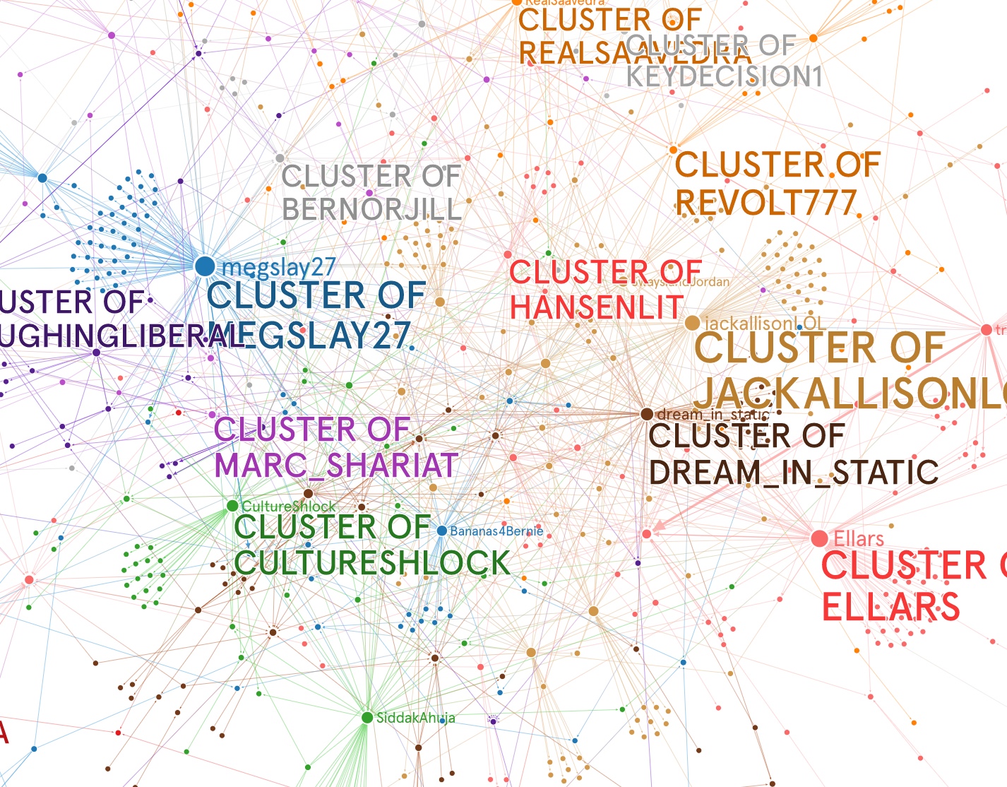
By far the conversation was dominated by one person. A next place to go is to see who these people are amplifying Bill Mitchell. We can do that with the Botometer. We can look at everyone involved in the conversation and score them for botlikeness. Here is an API that you can try, or use the Botometer by hand on their site.
# grab your keys from a previous notebook or https://apps.twitter.com

twitter_app_auth ={
"consumer_key" : "7iHkxooesKLdgQU5tFMfAtTZM",
"consumer_secret" : "GEivw4rYtMXcWNvO1fPg7GeEeNAofrLDul5fs2MqqEehfW9Alp"}#,
#"access_token" :"20743-l4HX83yCHL1K1QYFaYToNuXg6pHoYWXHDrmF4pbSq47y",
#"access_token_secret" : "bt4QJuiu8DygdpDJEQefPyuGGNwiUMBk74F7cKZKw0xa1"}


# here's my key - i'm not sure it will work for you or if it's tied to my twitter account
RapidKey = "28b5ce264amsh4634e3529278ab0p129fbejsn1a8530afc2dc"

from botometer import Botometer

botometer_api_url = 'https://botometer-pro.p.rapidapi.com'

meter = Botometer(botometer_api_url=botometer_api_url,
                  wait_on_ratelimit=True,
                  mashape_key=RapidKey,
                  **twitter_app_auth)
result = meter.check_account('HomebodyHeaven')
result
Another approach, had the conversation not been dominated by one person, would be to look at the network of people promoting a hashtag or a link or in some way moving the conversation forward. We did this for #MayorCheat in my class to great effect.